To the Moon Rocket Lab

Part 1
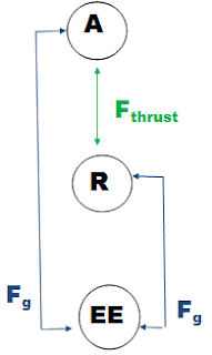
1. Draw a system schema  and force diagram  and apply Newton's Second Law to a rocket on the launch pad.

2. Redraw the system schema and force diagram and a statement of Newton's Second Law right based on this force diagram for the moment the rocket leaves the ground.

a. What agent is causing the upward force?

            The thrust force between the rocket and launch pad

b. Do you think the thrust force is constant? Explain
             Fnet = ma
             Fthrust - mg = ma
            Thrust force is not constant since it takes time for it to build up and your fuel level is changing over time.

3. As the fuel burns, is your rocket speeding up or slowing down? Which force has to be bigger for this to occur? Do you need to modify your force diagram?
             As fuel burns, our thrust force increases and our rocket looses mass, the force of gravity acting on the rocket is dependent on the mass (mg) therefore the rocket speeds up as it burns fuel. No need to modify force diagram

4. Your rocket is not a particle. Do you think you have to deal with air resistance? Redo your system schema, force diagram and statement of Newton's Second Law to include it.
              Yes air resistance is something we have to take into account

5. Do you think Fair is constant?  If not, what does it depend on?
               The force of air is not constant, it is dependent on the velocity of the rocket
               Fdrag = 1/4 Akv^2

6. When the rocket has run out of fuel, what direction is it still going? Is it speeding up or slowing down? Based on this what does your force diagram look like now. What is your new statement of Newton's Second Law?
                    It is still going up but it is slowing down.

7. How will you know when the rocket reaches its highest point?
              We know that the rocket reaches its max point once V = 0

8. What specific information and measurement do we need to calculate the maximum height the rocket reaches ?
              We will need the Force of gravity(Fg), mass of the rocket, our chance in time, density of air (rho), and the surface area of the rocket (A). We need to calculate for velocity, acceleration, air drag and change in position.

9.  Obtain the thrust vs time data for a rocket motor. Ultimately this data will be used to help calculate height of the rocket flight.

Part 2

For part 2 we actually went out and launched a model rocket, we then use the thrust from our rocket motor to solve for our max height. We knew that our initial values for our measurements were all zero. We also had our know values. We then use excel to solve for our maximum height by using our given values and our  equations for a, v, RhoAv^2, and r. Our max height came out to be approximately 146.85 m, which was really close to our given height of 147 m.

Conclusion:

This lab incorporated our knowledge on forces, drawing force diagrams, system schema, as well as using kinematic equations. We were able to figure out how to set up our problem by doing the system schema for our rocket then figuring out which equations to use so we can solve for our velocity, acceleration, air drag, and position. We were successful in this lab since we manage to acquire a .103% diff from our actual calculations compared to our theoretical. Over all this had to be one of the most challenging and fun labs this semester, since we really had to think about which values we had to calculate for first, then figure out where to go from there. The most fun was actually seeing the rocket model being launched as well as getting to work with all of our classmates on this lab since we could only launch one rocket. 

Lab 9: Human Power

Purpose:         To determine the power output of a person.

Equipment:    Two meter meter-sticks, stopwatch, and kilogram bathroom scale.

Introduction: Power is defined to be the rate at which work is done or equivalently, the rate at which energy is converted from one form to another. In this experiment you will do some work by climbing from the first floor of the science building to the second floor. By measuring the vertical height climbed and knowing you mass, the change in your gravitational potential energy can be found:

 △PE = mgh

        Where m is the mass, g the acceleration of gravity, and h is the vertical height gained.

         Your power output can be determined by

Power = △PE / △t   where △t is the time to climb the vertical height h.

Procedure:  We started this lab by recording our weight, which we then multiplied by g (9.8) to calculate for N. We measured the vertical distance between the ground floor and the second floor of the science building. The person keeping the time record for the class would time each persons running, or walking up the stairs. We did two trials. We then calculated our personal power output in watts using the data collected. We then determined our average power output in units of horsepower. Finally we added our average power on the board to calculate the average power of the entire class.

Data: 

 h = 4.26 m

mg = 860 N

t1= 8.25 s

t2= 8.16 s

Avg t = 8.21 s

△PE = mgh 

(860 kg*m/s^2) (4.26 m)

= 3,663. 6 kg*m^2/s^2

Power = △PE / △t

(3,663. 6 kg*m^2/s^2) / 8.21 s

= 446.24 W (1 Hp/ 746 W)

= .60 Hp

Questions: 1. Is it okay to use your hands and arms on the hand railing to assist you in your  

                       climb up the stairs? Explain why or why not.

                                 - Using the hand railing to assist is in going up the stairs is fine since it does not affect or change either your mass, the force of gravity or the height.

                   2. Discuss some of the problems with the accuracy of this experiment.

                              - A problem with accuracy might come from our measurements in height since it might be hard to get an accurate reading using only meter-sticks to measure. Our measurements for our weight and time might also not be as accurate as we might have wanted them to be.

  Conclusion: In this lab we learned about potential energy and power, and how potential energy could be defined as the energy that is within an object. Gravity gives the object its potential energy, which could be used to do work. Which is shown in our equation of PE = mgh. Power on the other hand is the rate at which the energy is used. Our equation for power shows us that while the same amount of work might be performed, if the change in time decreases more power is used, if the time increases then less power is used. 

Lab 7: Drag Force on a Coffee Filter

Purpose:         To study the relationship between air drag forces and the velocity of a falling    

                         body.

Equipment:    Computer with Logger Pro software, lab pro, motion detector, nine coffee filters,

                         meter stick.

Introduction: When an object moves through a fluid, such as air, it experiences a drag force that

                         opposes its motion. This force generally increases with velocity of the object. In

                         this lab we are going to investigate the velocity dependence of the drag force. We

                         will start by assuming the drag force, F_D, has a simple power law dependence on

                         the speed given by:

1)               F(drag) = k|v|^n, where the power n is to be determined by the experiment.

         This lab will investigate drag forces acting on a falling coffee filter. Because of the    

         large surface area and low mass of these filters, they reach terminal speed soon after

         being released.

Procedure: 
Note: You will be given a packet of nine nested coffee filters. It is important that the shape of this packet stays the same throughout the experiment so do not take the filters apart or otherwise alter the shape of the packet. Why is it important for the shape to stay the same? Explain and use a diagram. 

• Shape is important because the amount of drag produced depends on the surface area of the object. This way once the filters are released they accelerate until they reach terminal velocity.

1. Login to your computer with username and password. Start the Logger Pro software, open the

Mechanics folder and the graphlab file. Don’t forget to label the axes of the graph and create an appropriate title for the graph. Set the data collection rate to 30 Hz.

2. Place the motion detector on the floor facing upward and hold the packet of nine filters at a minimum height of 1.5 m directly above the motion detector. (Be aware other of nearby objects which can cause reflections.) Start the computer collecting data, and then release the packet. What should the position vs time graph look like? Explain.

• Our position vs time graph should show our object is decreasing in position while gaining speed  in the negative direction. Then it becomes linear to show it has reached terminal velocity, we know this since our slope would be constant, thus the linear graph.

Verify that the data are consistent. If not, repeat the trial. Examine the graph and using the mouse, select (click and drag) a small range of data points near the end of the motion where the packet moved with constant speed. Exclude any early or late points where the motion is not uniform.

3. Use the curve fitting option from the analysis menu to fit a linear curve (y = mx + b) to the selected data. Record the slope (m) of the curve from this fit. What should this slope represent? Explain.

• Our slope represents our terminal velocity since it's showing that our object is moving with a constant speed

Repeat this measurement at least four more times, and calculate the average velocity. Record all data in an excel data table.

4. Carefully remove one filter from the packet and repeat the procedure in parts 2 and 3 for the remaining packet of eight filters. Keep removing filters one at a time and repeating the above steps until you finish with a single coffee filter. Print a copy of one of your best x vs t graphs that show the motion and the linear curve fit to the data for everyone in your group (Do not include the data table; graph only please).

5. In Graphical Analysis, create a two column data table with packet weight (number of filters) in one column and average terminal speed (|v|) in the other. Make a plot of packet weight (y-axis) vs. terminal speed not velocity (x-axis). Choose appropriate labels and scales for the axes of your graph. Be sure to remove the “connecting lines” from the plot. Perform a power law fit of the  data and record the power, n, given by the computer. Obtain a printout of your graph for each member of your group. (Check the % error between your experimentally determined n and the theoretical value before you make a printout – you may need to repeat trials if the error is too large.)

% diff = |2 - 2.14 / 2 | x 100

 = 7 % diff

6. Since the drag force is equal to the packet weight, we have found the dependence of drag force on speed. Write equation 1 above with the value of n obtained from your experiment. Put a box around this equation. 

Drag = 1.90v^2.14

Look in the section on drag forces in your text and write down the equation given there for the drag force on an object moving through a fluid. How does your value of n compare with the value given in the text? What does the other fit parameter represent? Explain.

D= (1/4)A*v^2

We recorded our n to equal 2.14 which is close to the value that was given in the text of n=2. The other fit parameter represents the objects shape and and the density of the conditions which is moving through. The cross-section of our object is represented by A. 

Conclusion: In this lab we got a 7 % difference which shows that we weren't too far of from our accepted value. A cause for error could be that our coffee filters weren't neatly stacked so our drag force was not uniform. Another source of error came from using terminal speeds that were not consistent with out other trials, since our coffee filters wouldn't always land close to our motion detector.We also rounded our numbers so our calculations might not have been as accurate as we might have wanted them to be.

Lab 4: Working With Spreadsheets

Purpose: To get familiar with electronic spreadsheets by using them in some simple applications.

Equipment:  Computer with EXCEL software.

Introduction: For this lab we wanted to become familiarize with Excel since our labs expect us to collect data and using spreadsheets is a great way to keep our data collected and organized.

Procedure:  1. We started by opening the Excel software, then created a simple spreadsheet that calculates the values of the following function:

f (x) = A sin( Bx + C )

Our initial values given were

A= 5

B=3

C=(pi)/3

We placed our given values at the right side of the spreadsheet.

F(x) = A sin ( Bx+ C ) = $C$1*SIN(($E$1*A2)+$L$3)
Our Given Constants	Meaning of Each Constant		Cell Designation
A	Amplitude	5	C1
B	Frequency	3	E1
C	Phase	(pi)/3	G1
x	Radians	From 0-10 increments of 0.1	Columns A

After the data generated look presentable we then copied the data to the clipboard by highlighting the contents of the two columns and using EDIT/COPY from the menu bar. We then printed out a copy of our spreadsheet, as well as a spreadsheet formulas by using CTRL~

We then opened Graphical Analysis and copied our data onto the program. This allowed the program to graph the data we provided. Then we highlighted a portion of our graph, and using ANALYZE/CURVE FIT from the menu bar we picked the function

A*sinc (Bx + C) +D

to match the function we expected our data to match.

We repeated the process for a spreadsheet that calculates the position of a freely falling particle as a function of time. 

Rf= ½ aΔt^2 + V0Δt + ri = (0.5*$G$4)*((A2)^2)+($H$4*A2)+$I$4
Our Given Constants			Cell Designation
A	Acceleration of gravity	9.8 m/s^2	G4
B	Initial Velocity	50 m/s	H4
C	Initial Position	1000 m	I4
Δt	Time increment	0.2 sec (from 0-10 sec)	Columns A & D

Results:

Given	Results		Given	Results
A=5	5		A= -9.8	-4.9
B=3	3		B= 50	50
C= (pi)/3	1.407		C= 1000	1000

Conclusion: In this lab we learned how to manipulate our data so we are given a more precise reading when it comes to graphing, and organization. It was difficult at the beginning especially when we made errors by not putting the information in the correct column. By making the spreadsheet we were able to move that information into a different program, which we then used to get our constant, without having to do any calculations by hand. This method is helpful since we could also use it as a way to verify that our calculation are correct if we had tried to do the calculations by hand.   

Lab 1: Acceleration of Gravity

Purpose: The purpose of this lab is to determine the acceleration of gravity for a freely falling object. And to gain experience using the computer equipment to collect data.


Equipment: 

• Lab Pro interface

• Logger Pro software

• motion detector

• rubber ball

• wire basket

Introduction: In this laboratory you will use the computer to collect some position (x) vs time (t) data for a rubber ball tossed into the air. Since the velocity of an object is equal to the slope of the x vs t curve, the computer can also construct the graph of v vs t by calculating the slope of x vs t at each point in time. We will use both the x vs t graph and the v vs t graph to find the free fall acceleration of the ball.

Procedure: For this lab we first logged into Logger Pro to get a blank position vs. time graph. We had our position axes range from 0 to 4 (m), and our time axes range from 0 to 4 (s). We then hooked up our motion detector to Lab Pro interface, placed it on the floor and and put the wire basket above it, making sure that the wires of the basket weren't directly on top of the motion detector. While one member tossed the rubber ball up from about 1 m above the detector,  another member would  "collect" the data. The toss should have the ball going up then down directly above the detector for a more precise reading. We ran 3 trials, and for each of these trials we tried to get our position-time graph to be a parabolic shape since it would show the effect of gravity pulling the ball down when its tossed. After we had our data collected, we did a curve fit for the position vs. time graph for each trial to get an equation that would interpret the balls motion. 

Position-time graph

We used the quadratic fit (at^2 + bt + c) for our parabolic graph, equation , which gave us our values for a, b, and c. We used unit analysis to find the acceleration of our g exp for each trial. This was done by multiplying 2 to our a value given in our curve fit. We then calculated our percent difference percent to check how far off we were from getting the accepted value of gravity which is -9.8 m/s^2.

Velocity-time graph

After doing our curve fit we took a look at our velocity-time graph for the motion of our ball. We did a linear fit for this graph since we took the derivative of our position-time graph which gave us a linear graph for our velocity. The slope (m) of our graph gave us a close or equal measurement of -9.8 since the change in our velocity equals acceleration. Our acceleration of gravity came out as a negative value since the computer program read anything above our motion detector to be the positive direction and anything going down as our negative direction, and zero would be the position where our ball stopped going up and started to fall. Once we got our slope we calculated our percent difference.

Conclusion: In this lab we tracked the movement of a falling ball to solve for the acceleration of gravity. We  learned to read our position vs. time and velocity vs. time graphs. I also learn that for position graphs we are going to be given a parabolic graph since it shows the motion of our ball, while the velocity graph will be linear since the object in motion is uniform. Our results came really close to being exactly -9.8m/s^2. A source of error could be human error, as well as our motion detector recording outside interference which could have hampered our data since our ball wouldn't always land right on top of our motion detector.

Sample Post

Example of creating a function graph using graphical analysis